Model Specification using Rules

In this section, we now provide an informal description of the underlying model. The full details of this model can be found in (Schmidt 2012).

Tamarin models are specified using three main ingredients:

1. Rules
2. Facts
3. Terms

We have already seen the definition of terms in the previous section. Here we will discuss facts and rules, and illustrate their use with respect to the Naxos protocol, displayed below.

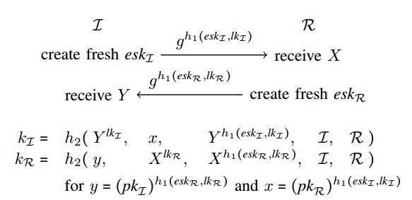
In this protocol, each party x has a long-term private key lkx and a corresponding public key pkx = 'g'^lkx, where 'g' is a generator of the Diffie-Hellman group. Because 'g' can be public, we model it as a public constant. Two different hash functions h1 and h2 are used.

To start a session, the initiator I first creates a fresh nonce eskI, also known as I’s ephemeral (private) key. He then concatenates eskI with I’s long-term private key lkI, hashes the result using the hash function h1, and sends 'g'^h1(eskI ,lkI) to the responder. The responder R stores the received value in a variable X, computes a similar value based on his own nonce eskR and long-term private key lkR, and sends the result to the initiator, who stores the received value in the variable Y. Finally, both parties compute a session key (kI and kR, respectively) whose computation includes their own long-term private keys, such that only the intended partner can compute the same key.

Note that the messages exchanged are not authenticated as the recipients cannot verify that the expected long-term key was used in the construction of the message. The authentication is implicit and only guaranteed through ownership of the correct key. Explicit authentication (e.g., the intended partner was recently alive or agrees on some values) is commonly achieved in authenticated key exchange protocols by adding a key-confirmation step, where the parties exchange a MAC of the exchanged messages that is keyed with (a variant of) the computed session key.

Rules

We use multiset rewriting to specify the concurrent execution of the protocol and the adversary. Multiset rewriting is a formalism that is commonly used to model concurrent systems since it naturally supports independent transitions.

A multiset rewriting system defines a transition system, where, in our case, the transitions will be labeled. The system’s state is a multiset (bag) of facts. We will explain the types of facts and their use below.

A rewrite rule in Tamarin has a name and three parts, each of which is a sequence of facts: one for the rule’s left-hand side, one labelling the transition (which we call ‘action facts’), and one for the rule’s right-hand side. For example:

rule MyRule1:
  [ ] --[ L('x') ]-> [ F('1','x'), F('2','y') ]

rule MyRule2:
  [ F(u,v) ] --[ M(u,v) ]-> [ H(u), G('3',h(v)) ]

For now, we will ignore the action facts (L(...) and M(...)) and return to them when discussing properties in the next section. If a rule is not labelled by action facts, the arrow notation --[ ]-> can be abbreviated to -->.

The rule names are only used for referencing specific rules. They have no specific meaning and can be chosen arbitrarily, as long as each rule has a unique name.

Executions

The initial state of the transition system is the empty multiset.

The rules define how the system can make a transition to a new state. A rule can be applied to a state if it can be instantiated such that its left hand side is contained in the current state. In this case, the left-hand side facts are removed from the state, and replaced by the instantiated right hand side.

For example, in the initial state, MyRule1 can be instantiated repeatedly.

For any instantiation of MyRule1, this leads to follow-up state that contains F('1','x') and F('2','y'). MyRule2 cannot be applied in the initial state since it contains no F facts. In the successor state, the rule MyRule2 can now be applied twice. It can be instantiated either by u equal to '1' (with v equal to 'x') or to '2' (with v equal to 'y'). Each of these instantiations leads to a new successor state.

Using ‘let’ binding in rules for local macros

When modeling more complex protocols, a term may occur multiple times (possibly as a subterm) within the same rule. To make such specifications more readable, Tamarin offers support for let ... in, as in the following example:

rule MyRuleName:
    let foo1 = h(bar)
        foo2 = <'bars', foo1>
        ...
        var5 = pk(~x)
    in
    [ ... ] --[ ... ]-> [ ... ]

Such let-binding expressions can be used to specify local term macros within the context of a rule. Each macro should occur on a separate line and defines a substitution: the left-hand side of the = sign must be a variable and the right-hand side is an arbitrary term. The rule will be interpreted after substituting all variables occurring in the let by their right-hand sides. As the above example indicates, macros may use the left-hand sides of earlier defined macros.

Global macros

Sometimes we want to use the same let binding(s) in multiples rules. In such a case, we can use the macros keyword to define global macros, which are applied to all rules. Consider the following example:

macros: macro1(x) = h(x), macro2(x, y) = <x, y>, ..., macro7() = $A

Here macro1 is the name of the first macro, and x is its the parameter. The second macro is called macro2 and has two parameters x and y. The last macro macro7 has no parameters. The the term on the right of the = sign is the output of the macro. It can be any term built from the functions defined in the equational theory and the parameters of the macro.

To use a macro in a rule, we can use the macro like a function inside terms. For example

[ In(macro1(~ltk)) ] --[ ... ]-> [ Out(macro2(pkA, pkB)) ]

will become

[ In(h(~ltk)) ] --[ ... ]-> [ Out(<pkA, pkB>) ]

after the above macros have been applied.

A macro can call a second macro, if the second one was defined before. For example, one can define the following two macros:

macros: innerMacro(x, y) = <x, y>, hashMacro(x, y) = h(innerMacro(x, y))

However, the following snippet would result in an error

macros: hashMacro(x, y) = h(innerMacro(x, y)), innerMacro(x, y) = <x, y>

as innerMacro is not yet defined when hashMacro is defined.

Macros only apply to rules, and are shown in interactive mode together with the protocol rules. When exporting a theory, Tamarin will export the original rules (before the macros were applied) and the macros.

Facts

Facts are of the form F(t1,...,tn) for a fact symbol F and terms ti. They have a fixed arity (in this case n). Note that if a Tamarin model uses the same fact with two different arities, Tamarin will report an error.

There are three types of special facts built in to Tamarin. These are used to model interaction with the untrusted network and to model the generation of unique fresh (random) values.

In

This fact is used to model a party receiving a message from the untrusted network that is controlled by a Dolev-Yao adversary, and can only occur on the left-hand side of a rewrite rule.

Out

This fact is used to model a party sending a message to the untrusted network that is controlled by a Dolev-Yao adversary, and can only occur on the right-hand side of a rewrite rule.

Fr

This fact must be used when generating fresh (random) values, and can only occur on the left-hand side of a rewrite rule, where its argument is the fresh term. Tamarin’s underlying execution model has a built-in rule for generating instances of Fr(x) facts, and also ensures that each instance produces a term (instantiating x) that is different from all others.

For the above three facts, Tamarin has built-in rules. In particular, there is a fresh rule that produces unique Fr(...) facts, and there is a set of rules for adversary knowledge derivation, which consume Out(...) facts and produce In(...) facts.

Linear versus persistent facts

The facts mentioned above are called ‘linear facts’. They are not only produced by rules, they also can be consumed by rules. Hence they might appear in one state but not in the next.

In contrast, some facts in our models will never be removed from the state once they are introduced. Modeling this using linear facts would require that every rule that has such a fact in the left-hand-side, also has an exact copy of this fact in the right-hand side. While there is no fundamental problem with this modeling in theory, it is inconvenient for the user and it also might lead Tamarin to explore rule instantiations that are irrelevant for tracing such facts in practice, which may even lead to non-termination.

For the above two reasons, we now introduce ‘persistent facts’, which are never removed from the state. We denote these facts by prefixing them with a bang (!).

Facts always start with an upper-case letter and need not be declared explicitly. If their name is prefixed with an exclamation mark !, then they are persistent. Otherwise, they are linear. Note that every fact name must be used consistently; i.e., it must always be used with the same arity, case, persistence, and multiplicity. Otherwise, Tamarin complains that the theory is not well-formed.

Comparing linear and persistent fact behaviour we note that if there is a persistent fact in some rule’s premise, then Tamarin will consider all rules that produce this persistent fact in their conclusion as the source. Usually though, there are few such rules (most often just a single one), which simplifies the reasoning. For linear facts, particularly those that are used in many rules (and kept static), obviously there are many rules with the fact in their conclusion (all of them!). Thus, when looking for a source in any premise, all such rules need to be considered, which is clearly less efficient and non-termination-prone as mentioned above. Hence, when trying to model facts that are never consumed, the use of persistent facts is preferred.

Embedded restrictions

A frequently used trick when modelling protocols is to enforce a restriction on the trace once a certain rule is invoked, for instance if the step represented by the rule requires another step at some later point in time, e.g., to model a reliable channel. We explain what restriction are later, but roughly speaking, they specify constraints that a protocol execution should uphold.

This can be done by hand, namely by specifying a restriction that refers to an action fact unique to this rule, or by using embedded restrictions like this:

rule B:
    [In(x), In(y)] --[ _restrict( formula )]-> []

where formula is a restriction. Note that embedded restrictions currently are only available in trace mode.

Modeling protocols

There are several ways in which the execution of security protocols can be defined, e.g., as in (Cremers and Mauw 2012). In Tamarin, there is no pre-defined protocol concept and the user is free to model them as she or he chooses. Below we give an example of how protocols can be modeled and discuss alternatives afterwards.

Public-key infrastructure

In the Tamarin model, there is no pre-defined notion of public key infrastructure (PKI). A pre-distributed PKI with asymmetric keys for each party can be modeled by a single rule that generates a key for a party. The party’s identity and public/private keys are then stored as facts in the state, enabling protocol rules to retrieve them. For the public key, we commonly use the Pk fact, and for the corresponding long-term private key we use the Ltk fact. Since these facts will only be used by other rules to retrieve the keys, but never updated, we model them as persistent facts. We use the abstract function pk(x) to denote the public key corresponding to the private key x, leading to the following rule. Note that we also directly give all public keys to the attacker, modeled by the Out on the right-hand side.

rule Generate_key_pair:
  [ Fr(~x) ]
  -->
  [ !Pk($A,pk(~x))
  , Out(pk(~x))
  , !Ltk($A,~x)
  ]

Some protocols, such as Naxos, rely on the algebraic properties of the key pairs. In many DH-based protocols, the public key is \(g^x\) for the private key \(x\), which enables exploiting the commutativity of the exponents to establish keys. In this case, we specify the following rule instead.

rule Generate_DH_key_pair:
  [ Fr(~x) ]
  -->
  [ !Pk($A,'g'^~x)
  , Out('g'^~x)
  , !Ltk($A,~x)
  ]

Modeling a protocol step

Protocols describe the behavior of agents in the system. Agents can perform protocol steps, such as receiving a message and responding by sending a message, or starting a session.

Modeling the Naxos responder role

We first model the responder role, which is simpler than the initiator role since it can be done in one rule.

The protocol uses a Diffie-Hellman exponentiation, and two hash functions h1 and h2, which we must declare. We can model this using:

builtins: diffie-hellman

and

functions: h1/1
functions: h2/1

Without any further equations, a function declared in this fashion will behave as a one-way function.

Each time a responder thread of an agent $R receives a message, it will generate a fresh value ~eskR, send a response message, and compute a key kR. We can model receiving a message by specifying an In fact on the left-hand side of a rule. To model the generation of a fresh value, we require it to be generated by the built-in fresh rule.

Finally, the rule depends on the actor’s long-term private key, which we can obtain from the persistent fact generated by the Generate_DH_key_pair rule presented previously.

The response message is an exponentiation of g to the power of a computed hash function. Since the hash function is unary (arity one), if we want to invoke it on the concatenation of two messages, we model them as a pair <x,y> which will be used as the single argument of h1.

Thus, an initial formalization of this rule might be as follows:

    rule NaxosR_attempt1:
            [
              In(X),
              Fr(~eskR),
              !Ltk($R, lkR)
            ]
            -->
            [
              Out( 'g'^h1(< ~eskR, lkR >) )
            ]

However, the responder also computes a session key kR. Since the session key does not affect the sent or received messages, we can omit it from the left-hand side and the right-hand side of the rule. However, later we will want to make a statement about the session key in the security property. We therefore add the computed key to the actions:

    rule NaxosR_attempt2:
            [
              In(X),
              Fr(~eskR),
              !Ltk($R, lkR)
            ]
            --[ SessionKey($R, kR ) ]->
            [
              Out( 'g'^h1(< ~eskR, lkR >) )
            ]

The computation of kR is not yet specified in the above. We could replace kR in the above rule by its full unfolding, but this would decrease readability. Instead, we use let binding to avoid duplication and reduce possible mismatches. Additionally, for the key computation we need the public key of the communication partner $I, which we bind to a unique thread identifier ~tid; we use the resulting action fact to specify security properties, as we will see in the next section. This leads to:

    rule NaxosR_attempt3:
      let
          exR = h1(< ~eskR, lkR >)
          hkr = 'g'^exR
          kR  = h2(< pkI^exR, X^lkR, X^exR, $I, $R >)
      in
       [
           In(X),
           Fr( ~eskR ),
           Fr( ~tid ),
           !Ltk($R, lkR),
           !Pk($I, pkI)
       ]
       --[ SessionKey( ~tid, $R, $I, kR ) ]->
       [
           Out( hkr )
       ]

The above rule models the responder role accurately, and computes the appropriate key.

We note one further optimization that helps Tamarin’s backwards search. In NaxosR_attempt3, the rule specifies that lkR might be instantiated with any term, hence also non-fresh terms. However, since the key generation rule is the only rule that produces Ltk facts, and it will always use a fresh value for the key, it is clear that in any reachable state of the system, lkR can only become instantiated by fresh values. We can therefore mark lkR as being of sort fresh, therefore replacing it by ~lkR.¹

rule NaxosR:
  let 
      exR = h1(< ~eskR, ~lkR >)
      hkr = 'g'^exR
      kR  = h2(< pkI^exR, X^~lkR, X^exR, $I, $R >)
  in
   [
       In(X),
       Fr( ~eskR ),
       Fr( ~tid ),
       !Ltk($R, ~lkR),
       !Pk($I, pkI)
   ]
   --[ SessionKey( ~tid, $R, $I, kR ) ]->
   [
       Out( hkr )
   ]

The above rule suffices to model basic security properties, as we will see later.

Modeling the Naxos initiator role

The initiator role of the Naxos protocol consists of sending a message and waiting for the response. While the initiator is waiting for a response, other agents might also perform steps. We therefore model the initiator using two rules.²

The first rule models an agent starting the initiator role, generating a fresh value, and sending the appropriate message. As before, we use let binding to simplify the presentation and use ~lkI instead of lkI since we know that !Ltk facts are only produced with a fresh value as the second argument.

    rule NaxosI_1_attempt1:
      let exI = h1(<~eskI, ~lkI >)
          hkI = 'g'^exI
      in
       [   Fr( ~eskI ),
           !Ltk( $I, ~lkI ) ]
       -->
       [   Out( hkI ) ]

Using state facts to model progress

After triggering the previous rule, an initiator will wait for the response message. We still need to model the second part, in which the response is received and the key is computed. To model the second part of the initiator rule, we must be able to specify that it was preceded by the first part and with specific parameters. Intuitively, we must store in the state of the transition system that there is an initiator thread that has performed the first send with specific parameters, so it can continue where it left off.

To model this, we introduce a new fact, which we often refer to as a state fact: a fact that indicates that a certain process or thread is at a specific point in its execution, effectively operating both as a program counter and as a container for the contents of the memory of the process or thread. Since there can be any number of initiators in parallel, we need to provide a unique handle for each of their state facts.

Below we provide an updated version of the initiator’s first rule that produces a state fact Init_1 and introduces a unique thread identifier ~tid for each instance of the rule.

rule NaxosI_1:
  let exI = h1(<~eskI, ~lkI >)
      hkI = 'g'^exI
  in
   [   Fr( ~eskI ),
       Fr( ~tid ),
       !Ltk( $I, ~lkI ) ]
   -->
   [   Init_1( ~tid, $I, $R, ~lkI, ~eskI ),
       Out( hkI ) ]

Note that the state fact has several parameters: the unique thread identifier ~tid³, the agent identities $I and $R, and the actor’s long-term private key ~lkI, and the private exponent. This now enables us to specify the second initiator rule.

rule NaxosI_2:
  let
      exI = h1(< ~eskI, ~lkI >)
      kI  = h2(< Y^~lkI, pkR^exI, Y^exI, $I, $R >)
  in
   [   Init_1( ~tid, $I, $R, ~lkI , ~eskI),
       !Pk( $R, pkR ),
       In( Y ) ]
   --[ SessionKey( ~tid, $I, $R, kI ) ]->
  []

This second rule requires receiving a message Y from the network but also that an initiator fact was previously generated. This rule then consumes this fact, and since there are no further steps in the protocol, does not need to output a similar fact. As the Init_1 fact is instantiated with the same parameters, the second step will use the same agent identities and the exponent exI computed in the first step.

Thus, the complete example becomes:

theory Naxos
begin

builtins: diffie-hellman

functions: h1/1
functions: h2/1

rule Generate_DH_key_pair:
  [ Fr(~x) ] 
  --> 
  [ !Pk($A,'g'^~x)
  , Out('g'^~x)
  , !Ltk($A,~x)
  ]

rule NaxosR:
  let 
      exR = h1(< ~eskR, ~lkR >)
      hkr = 'g'^exR
      kR  = h2(< pkI^exR, X^~lkR, X^exR, $I, $R >)
  in
   [
       In(X),
       Fr( ~eskR ),
       Fr( ~tid ),
       !Ltk($R, ~lkR),
       !Pk($I, pkI)
   ]
   --[ SessionKey( ~tid, $R, $I, kR ) ]->
   [
       Out( hkr )
   ]

rule NaxosI_1:
  let exI = h1(<~eskI, ~lkI >)
      hkI = 'g'^exI
  in
   [   Fr( ~eskI ),
       Fr( ~tid ),
       !Ltk( $I, ~lkI ) ]
   -->
   [   Init_1( ~tid, $I, $R, ~lkI, ~eskI ),
       Out( hkI ) ]

rule NaxosI_2:
  let
      exI = h1(< ~eskI, ~lkI >)
      kI  = h2(< Y^~lkI, pkR^exI, Y^exI, $I, $R >)
  in
   [   Init_1( ~tid, $I, $R, ~lkI , ~eskI),
       !Pk( $R, pkR ),
       In( Y ) ]
   --[ SessionKey( ~tid, $I, $R, kI ) ]->
  []

end

Note that the protocol description only specifies a model, but not which properties it might satisfy. We discuss these in the next section.

---

1. Note that in contrast, replacing X by ~X would change the interpretation of the model, effectively restricting the instantiations of the rule to those where X is a fresh value.↩︎

2. This modeling approach, as with the responder, is similar to the approach taken in cryptographic security models in the game-based setting, where each rule corresponds to a “query”.↩︎

3. Note that we could have re-used ~eskI for this purpose, since it will also be unique for each instance.↩︎